The Moving Average Strategy

If you read all three blog posts so far I want to thank but also congratulate you! Because you’ve gained fundamental and powerful investment knowledge backed by research and data. Factual knowledge!

Previously...

In the first post “Let’s talk about ‘Buy and Hold’” we calculated that the SPY returned 10.4% annually on average over the last 30 years but learned also about the "Lost Decade" problem. Then we understood that we can boost our "Buy and Hold" with Dollar Cost Averaging (DCA)" and buy every month SPY for $200.

We defined our first "algorithmic" investment strategy:

"In addition to our initial $10,000 SPY investment we buy every first workday of the month SPY ETFs for $200 - rain or sunshine."

This helped us tremendously in tough periods like the "Lost Decade" where we still increased our portfolio because we bought SPY every month. And last week we looked closely into an important issue when investing - Volatility!

Benchmark

Today we use the "Buy and Hold" with Dollar Cost Averaging (DCA)" as our benchmark and test if we can make it better.

What is the Sharpe Ratio?

Before we improve a strategy we need to know what we want to improve. Do we want to increase our return or reduce our risk? Or both?

Instinctively we know as investors that we have to accept risk in order to get return. No risk no fun! No pain no gain! Everyone knows that.

In 1966 William F. Sharpe created what he called the "reward-to-variability ratio" (later named the Sharpe Ratio) to measure the risk/fun or pain/gain factor for investing. Basically the Sharpe Ratio will enable us to compare investments and tell us which of the investments we get paid the most for the risk we are taking. After all you don't want to take unnecessary risks!

The Sharpe Ratio is calculated as:

$$ \text{Sharpe Ratio} = \frac{R_p - R_f}{\sigma_p} $$

Where:

• \( R_p \) = Return of the portfolio or investment
• \( R_f \) = Risk-free rate (such as the return on government bonds)
• \( \sigma_p \) = Standard deviation (volatility) of the portfolio’s returns

The Sharpe Ratio helps us understand the return we are getting relative to the risk we are taking. A higher Sharpe Ratio means better risk-adjusted returns, and it’s useful for comparing different investments.

Excellent! Now let the fun begin!

The Moving Average Strategy

Ladies and gentlemen may I introduce the "Moving Average Strategy".

So far we always stayed invested in the SPY and bought every month additional SPY for $200. After all it's called the "Buy and Hold" strategy for a reason! Don't let go!!!

With the "Moving Average Strategy" we will learn to let go. Yes! Sometimes you need to let go. Remember Elsa in the Disney movie Frozen? "Let it go!". She knows!

In order to know when to say goodby to the SPY we do a simple calculation every month and depending on the result we do either A or B.

A) Continue and buy SPY for an additional $200

B) Stop and sell all SPYs we have and keep cash in our account

This is not complicated and since we only do that once a month it's not time consuming at all. Do we have a new strategy?

Sure we do! Let's call it for simplicity the "Moving Average Strategy" and let's put it to the test!

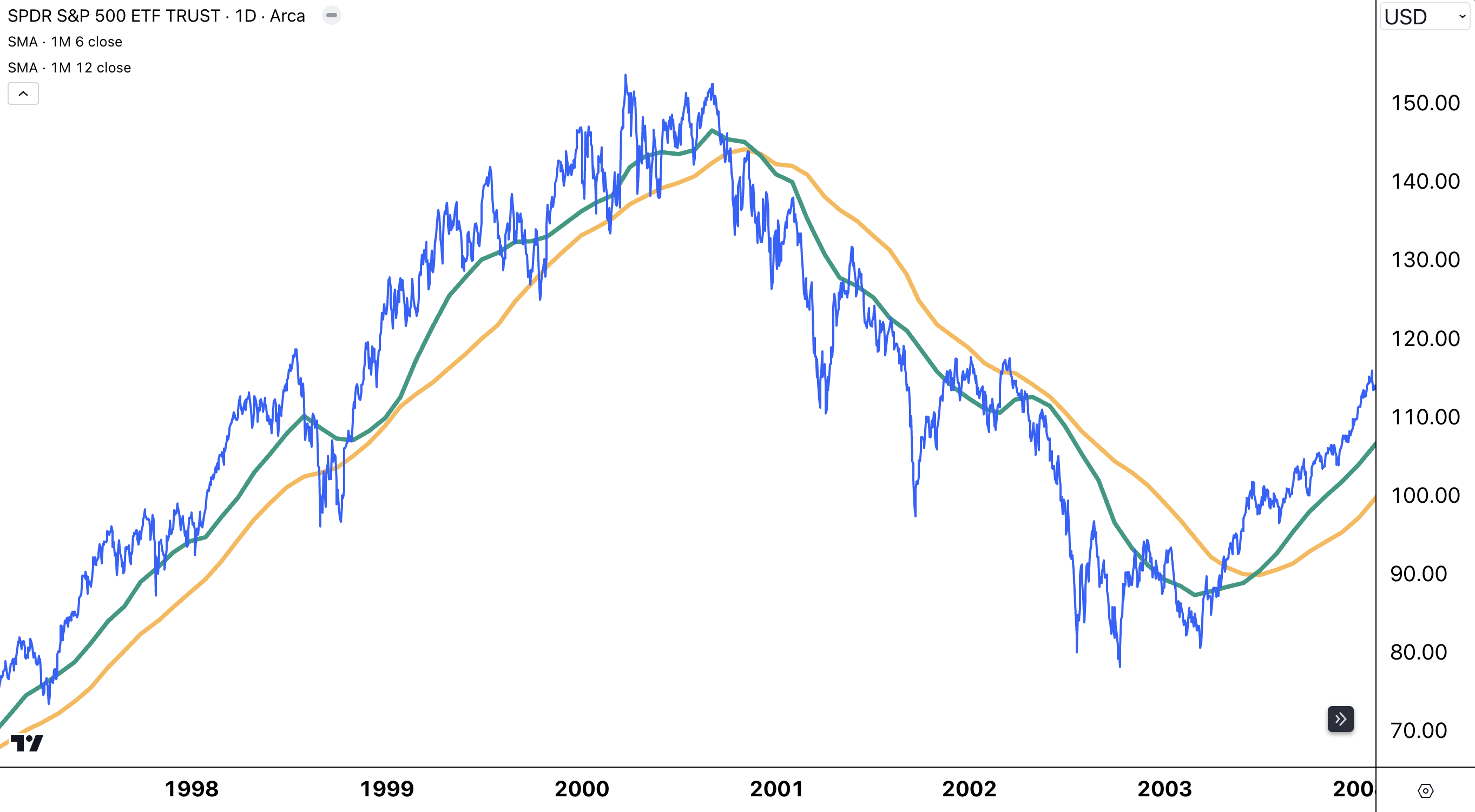
Here we see the daily SPY prices in blue and the 12 month average in orange and the 6 month average in green.^[1]

Our rule is simple - every month we check where the green line is in relation to the orange line. The green 6 month moving average is above the orange 12 month moving average and we buy SPY with our $200 savings. But if the green 6 month moving average line is below the orange 12 month moving average line we sell all SPY we have and keep the cash in our account until the green line is above the orange line again. Simple? Sure it is simple. Thats the beauty!

It looks good on the chart but did it really work?

The Backtest

When we ask "Did it really work?" we could ask "Is the Sharpe Ratio of our new strategy higher than our benchmark. Let's look at the backtest over almost 30 years from Jan 1995 until Aug 2024. I am using a service here called Portfolio Visualizer. We are not getting sponsored nor is this an affiliate link. But I think this is a good starting point to test some investment strategies and do some research.

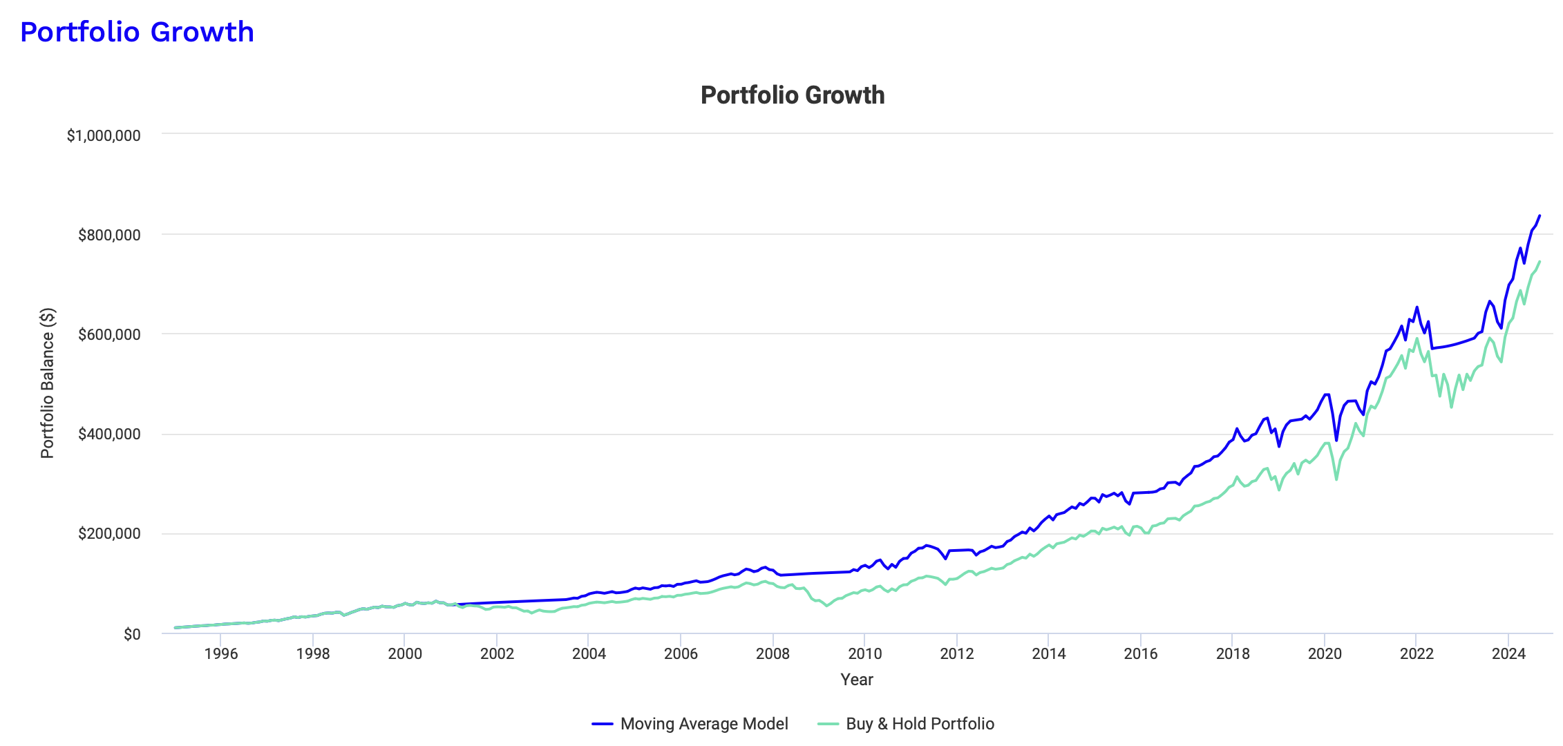
When we look closer we see that the blue line - our moving average strategy - does quite well and did not suffer as many down moves compared to the green buy and hold benchmark. Let's look at some performance statistics.

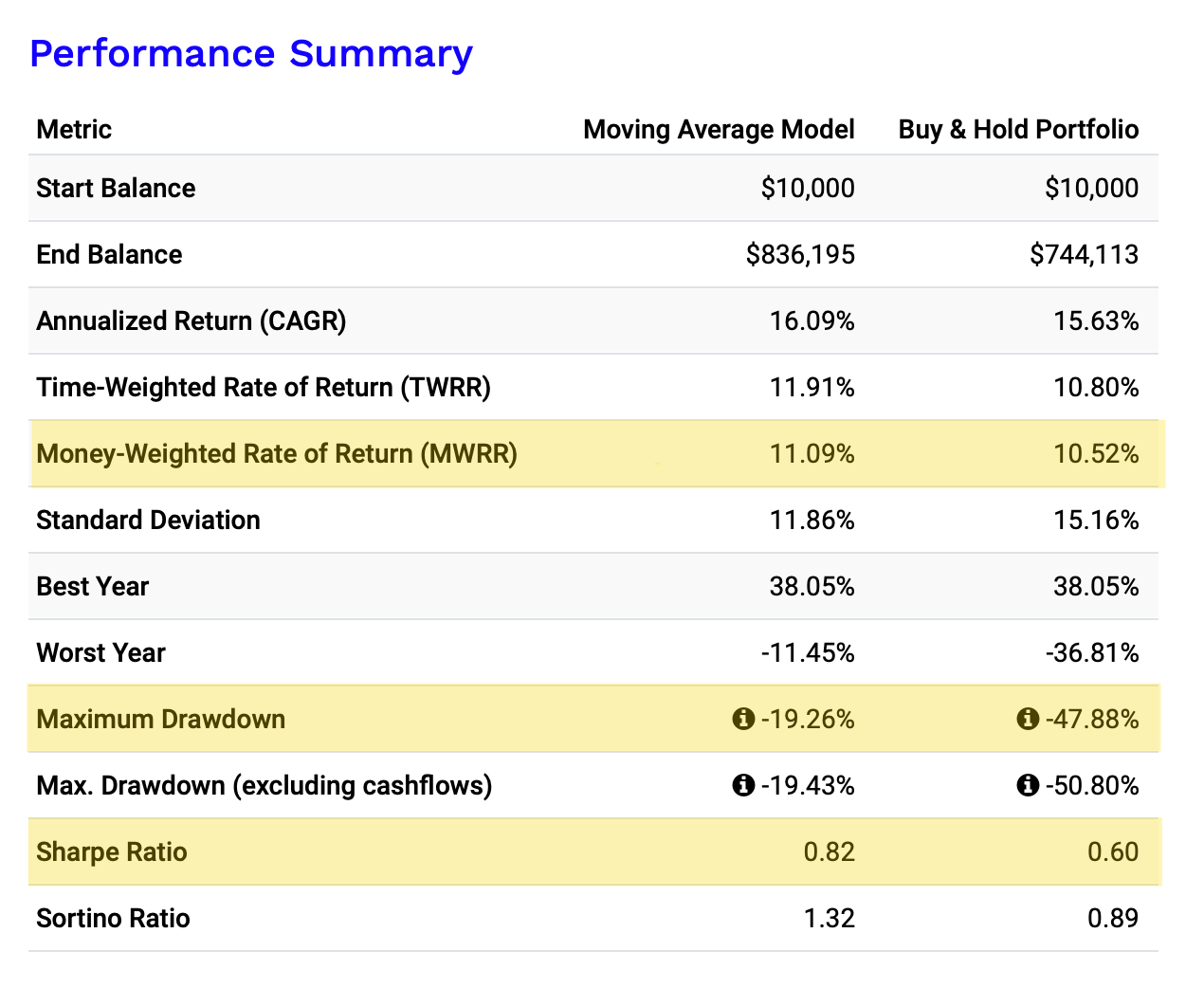
The return^[2] of the benchmark strategy is 10.5% compared to our new moving average strategy of 11%. Our new strategy has a slightly higher return, What’s the Sharpe Ratio, you ask? I am so proud of you! Yes, that's the important question! The Sharpe Ratio moved up from 0.6 to 0.82. This is a 36% increase. Fantastic! We are now taking less risk for almost the same return.

When looking at the Maximum Drawdown which measure the the biggest percentage drop in our portfolio value over a single month, it becomes very clear that we are taking less risk. The worst drawdown of the benchmark was 47% and only 19% of the moving average strategy.

If you say : "Same return, less max drawdown and higher Sharpe. - I love it!". I would agree with you.

By the way if we want to start a hedge fund with our strategies, we need to get at least above a Sharpe ratio of around 1 and ideally above 1.5 in order for investors to return our call.

Zooming into the 2000-2010 period of the "Lost Decade" we can see how our strategy saved us quite some pain.

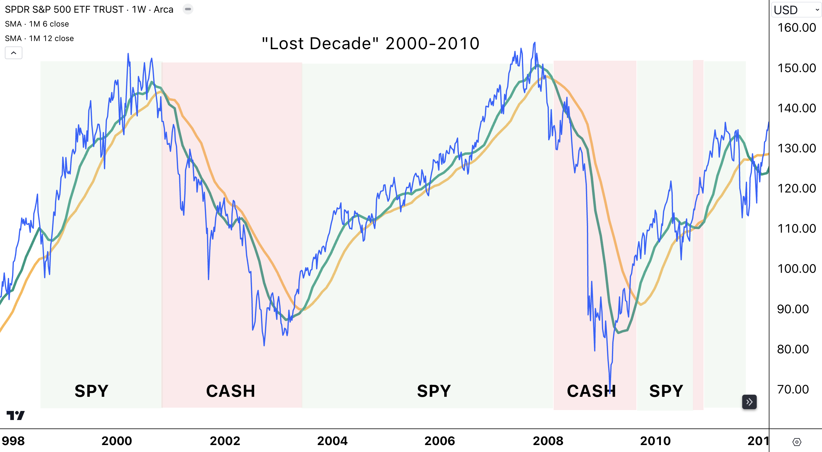
End of 2000 the green line moved below the orange line and this is where we sold all our SPY and kept cash (red box) until mid of 2003. We had to wait 2.5 years before the green line moved above the orange line again and we invested all our cash into SPY. Then in February 2008 the green line moved below the orange line again and we sold all SPY until September 2009 our signal reverses and we invested all our cash in SPY.

Is this too good to be true?

Always be skeptical and question everything! When we use different moving averages instead of the 6 and 12 month we get similar results, but if we use too short or too long averages the Sharpe improvements are less significant.

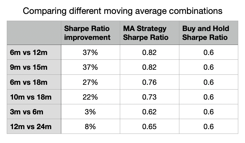
How much we can improve our risk/reward ratio depends on what moving averages we use for our monthly signal. At this point we need to talk about a real problem with backtesting. Let me tell you, it is a real party pooper! It is called "Overfitting".

Over-What?

Let's ChatGPT explain you what overfitting is.

Overfitting in backtesting happens when a trading strategy is too closely tailored to past data, making it look great in hindsight but not perform well in the future.

Here’s a simple analogy: Imagine you’re studying for a test. Instead of learning the general concepts, you memorize all the answers to last year’s exam. You might do perfectly on that specific test, but if the questions change even a little on this year’s test, you might fail because you didn’t really learn the material.

In backtesting, overfitting is like “memorizing” the past market data too closely. The strategy is designed to work perfectly with historical data, but it becomes too specific to patterns that may not repeat. As a result, it doesn’t perform well when applied to new, unseen market conditions.

Great explanation! Thank you ChatGPT!

Great! What do we do now?

Overfitting is an issue we have to keep in mind before implementing a strategy in real life with real money. There are things we can do to reduce the risk of overfitting. We’ll discuss them in later posts. But for now these backtests are the least we can do? Why would we ever follow an investment strategy that never worked in the past?

Conclusion

With this moving average strategy we have outperformed our benchmark. We get a similar return and we took far less risk. The higher Sharpe ratio shows that.

In general, moving averages play a very important role in many investment and trading strategies used by professional investment managers. Not in this simple form but very similar.

If you’re interested in taking this further, we’ll eventually explore how machine learning can enhance a simple moving average strategy. Don’t worry if you’re not familiar with machine learning yet—we'll dedicate a separate post to explain it in detail. Later, we’ll dive into how various techniques like grid search, random search, genetic algorithms, Bayesian optimization, and walk-forward optimization can automate and optimize the strategy. It may sound complicated, but I promise it’s more straightforward than it seems. Trust me, I’m not a math geek either!

Congratulations! This is your third investment strategy. Well done!

Until next week where we use historical data to make a simulation of our portfolio value in the future. All we need is 1.21 gigawatts and a flux capacitor.

Footnotes

^[1] We use here a simple moving average. Every month we add the last 12 monthly SPY prices and divide them by 12 and do the same for the last 6 month. There are many other types of moving averages you might want to explore and test. Ask your favorite AI tool about Exponential Moving Average (EMA), Weighted Moving Average (WMA), Hull Moving Average (HMA), Kaufman’s Adaptive Moving Average (KAMA) and Triangular Moving Average (TMA).

^[2] There are several ways to calculate a return, here we use the Money-Weighted Rate of Return to take into account that we invest every month.